Datos y Mezcales
En el marco del Festival LATAM de Medios Digitales y Periodismo, por Factual y Distintas Latitudes.
26 y 27 de Octubre del 2023
Desplazamiento climático: La migración que no vemos.
Un trabajo de N+ Focus.

![]()


Holi
¿Quién soy?
Me llamo Isaac Arroyo, y aquí unos puntos rápidos sobre mi:
- Casi siempre estoy escuchando música de Alessia Cara, Taylor Swift, Calle 13 y últimamente Kendrick Lamar.
- Soy ingeniero físico pero no me veo didicándome a la física ni a la ingeniería.
- Mi sueño es tener una cafetería pero no tengo el dinero para empezarla. En lo que junto dinero, me dedico haciendo todo lo que se pueda hacer con los datos en N+ Focus, la unidad de periodismo de investigación de N+.
Desplazamiento climático: La migración que no vemos
¿De qué va?
Narra las historias de las personas que han tenido que dejar su hogar, su estado o el país por las consecuencias de la emergencia climática.

Imagen tomada del trabajo interactivo “Desplazamiento climático: La migración que no vemos”
La sequía de la Laguna de Metztitlán, Hidalgo.
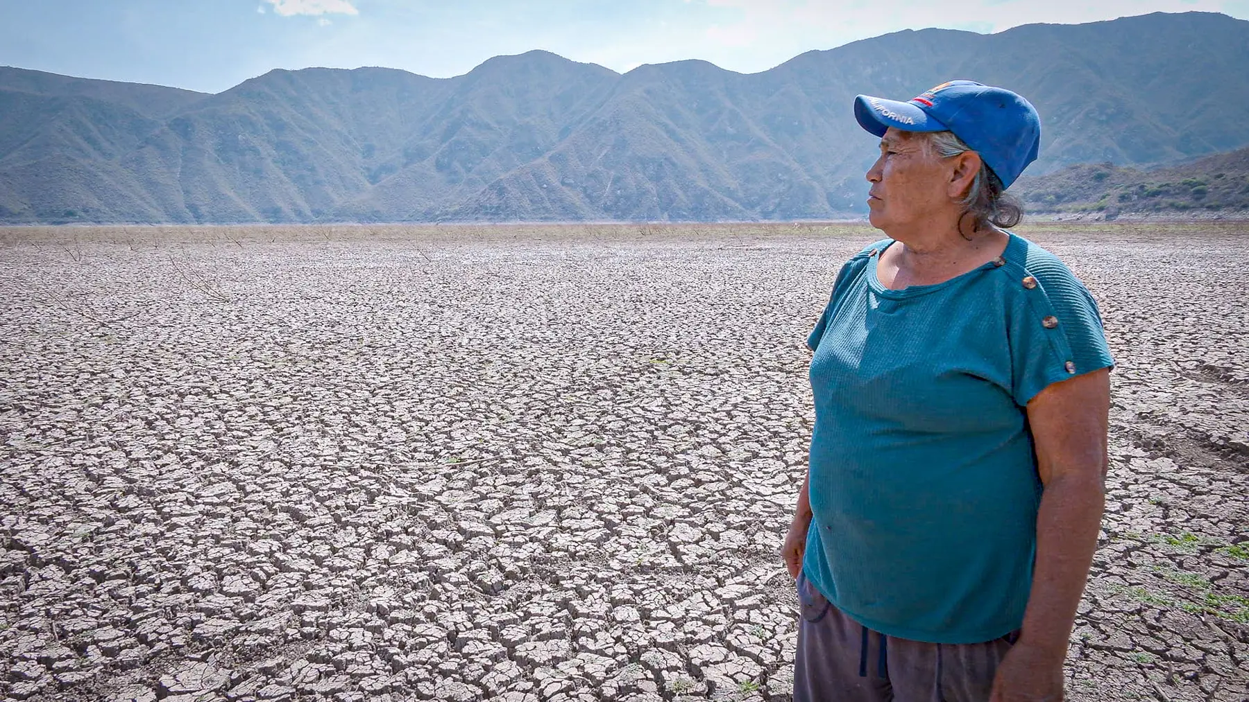
Imagen tomada del trabajo interactivo “Desplazamiento climático: La migración que no vemos”
El aumento del nivel del mar en la comunidad de El Bosque, Tabasco.

Imagen tomada del trabajo interactivo “Desplazamiento climático: La migración que no vemos”
La falta de lluvias en Santiago Pinotepa Nacional, Oaxaca.

Imagen tomada del trabajo interactivo “Desplazamiento climático: La migración que no vemos”
En el reportaje interactivo puedes jugar con las visualizaciones y los mapas1
El reto de los datos
Registros antiguos que cubran cada rincón del país
Parte fundamental del trabajo era encontrar regiones que hayan sido afectadas por la crisis climática… y la verdad, todo el mundo esta siendo afectado por la crisis climática, unos más que otros.
Además, platicando con expertos en el tema, recomendaron tener datos que tengan como mínimo 30 años de antigüedad, esto para poder observar y calcular las anomalías1
¿La solución?
TerraClimate y Google Earth Engine
Google Earth Engine es una plataforma que facilita1 el acceso a datos raster e imágenes satelitales.
Dentro de su catálogo de datos se encuentra TerraClimate, un conjunto de datos de reconstrucciones2 del clima

De imágenes a tabla
Agarrar las imágenes y llevar los valores a una tabla tomó muchos intentos, mucha lectura de documentación, y también mucho café, pero al final se logró.
Imágenes ➜ Tabla Pt. I
import ee
import geemap
ee.Initialize()
print("Earth Engine inicializado")
print("Empieza a correr el código...")

# = = = = Valores variables = = = = = =
banda_interes = "pdsi"
type_of_geometry = "ent"
type_reducer_time = "year"
temp_zscore = False

# - - - - - - - - - - - - - - - - - - - - -
# banda_interes
dict_functions_scalling_var_int = {
    "pdsi": {
        "scalling_func" : lambda img: img.multiply(0.01).copyProperties(img, img.propertyNames()),
        "var_int_func": lambda img: img.copyProperties(img, img.propertyNames()),
    },
    "pr": {
        "scalling_func": lambda img: img.copyProperties(img, img.propertyNames()),
        "var_int_func": lambda img: img.subtract(mean_base_months).divide(mean_base_months).copyProperties(img, img.propertyNames())
    },
    "tmmx": {
        "scalling_func": lambda img: img.multiply(0.1).copyProperties(img, img.propertyNames()),
        "var_int_func": lambda img: img.subtract(mean_base_months).copyProperties(img, img.propertyNames()),
        "var_int_func_zscore": lambda img: img.subtract(mean_base_months).divide(std_base_months).copyProperties(img, img.propertyNames())
    },
    "tmmn": {
        "scalling_func": lambda img: img.multiply(0.1).copyProperties(img, img.propertyNames()),
        "var_int_func": lambda img: img.subtract(mean_base_months).copyProperties(img, img.propertyNames()),
        "var_int_func_zscore": lambda img: img.subtract(mean_base_months).divide(std_base_months).copyProperties(img, img.propertyNames())
    }
}

# type_of_geometry
if type_of_geometry == "mun":
    # Municipios
    fc = ee.FeatureCollection("projects/ee-unisaacarroyov/assets/GEOM-MX/MX_MUN_2022")
elif type_of_geometry == "ent":
    # Estados
    fc = ee.FeatureCollection("projects/ee-unisaacarroyov/assets/GEOM-MX/MX_ENT_2022")
elif type_of_geometry == "nac":
    # Nación
    fc = ee.FeatureCollection("USDOS/LSIB/2017").filter(ee.Filter.eq("COUNTRY_NA","Mexico"))

# type_reducer_time
dict_reducers = {
    "month": lambda number: final_data_img_coll
                            .filter(ee.Filter.eq("date_year", number))\
                            .first()\
                            .reduceRegions(reducer = ee.Reducer.mean(), collection = fc, scale = scale_img_coll)\
                            .map(lambda feature: ee.Feature(feature).set("date_year", number).setGeometry(None)),
    "year": lambda number: final_data_img_coll
                           .filter(ee.Filter.eq("date_year", number))\
                           .first()\
                           .reduce(ee.Reducer.mean())\
                           .reduceRegions(reducer = ee.Reducer.mean(), collection = fc, scale = scale_img_coll)\
                           .map(lambda feature: ee.Feature(feature).set("date_year", number).setGeometry(None))
}


# = = = = Valores constantes = = = = =
img_coll = ee.ImageCollection("IDAHO_EPSCOR/TERRACLIMATE")
geom_mex = ee.FeatureCollection("USDOS/LSIB/2017").filter(ee.Filter.eq("COUNTRY_NA","Mexico")).first().geometry()
scale_img_coll = 4638.3
start_date_base = "1960-01-01"
end_date_base = "1989-12-31"
img_coll_start_year = 1960
img_coll_end_year = 2022
n_max_features = 3000

# - - Valor "constante" - - - - -
str_folder = "name_of_folder"


# = = = = Funciones escenciales = = = = = =

def tag_month_year(img):
    full_date = ee.Date(ee.Number(img.get("system:time_start")))
    date_year = ee.Number(full_date.get("year"))
    date_month = ee.Number(full_date.get("month"))
    return img.set({"date_month": date_month, "date_year": date_year})

def func_base_mean(element):
    return data_image_coll_tag_year_month.filterDate(start_date_base, end_date_base).filter(ee.Filter.eq("date_month", element)).mean().set({"date_month": element})

def func_base_std(element):
    return data_image_coll_tag_year_month.filterDate(start_date_base, end_date_base).filter(ee.Filter.eq("date_month", element)).reduce(ee.Reducer.stdDev()).set({"date_month": element})

# = = = =  INICIO DE CÓDIGO  = = = = = = = =

data_image_coll_tag_year_month = img_coll.select(banda_interes).filter(ee.Filter.bounds(geom_mex)).map(dict_functions_scalling_var_int[banda_interes]["scalling_func"]).map(tag_month_year)

# Media historica
list_img_to_img_coll_base_mean_months = ee.List.sequence(1,12,1).map(func_base_mean)
mean_base_months = ee.ImageCollection.fromImages(list_img_to_img_coll_base_mean_months).toBands().rename(["01","02","03","04","05","06","07","08","09","10","11","12"])

# std historica
list_img_to_img_coll_base_std_months = ee.List.sequence(1,12,1).map(func_base_std)
std_base_months = ee.ImageCollection.fromImages(list_img_to_img_coll_base_std_months).toBands().rename(["01","02","03","04","05","06","07","08","09","10","11","12"])

list_new_collection_by_year = ee.List.sequence(img_coll_start_year, img_coll_end_year).map(lambda element: data_image_coll_tag_year_month.filter(ee.Filter.eq("date_year", element)).toBands().set({"date_year": element}).rename(["01","02","03","04","05","06","07","08","09","10","11","12"]))

if temp_zscore == False:
    final_data_img_coll = ee.ImageCollection.fromImages(list_new_collection_by_year).map(dict_functions_scalling_var_int[banda_interes]["var_int_func"])
elif temp_zscore == True:
    final_data_img_coll = ee.ImageCollection.fromImages(list_new_collection_by_year).map(dict_functions_scalling_var_int[banda_interes]["var_int_func_zscore"])

list_fc_from_img_coll = ee.List.sequence(img_coll_start_year, img_coll_end_year).map(dict_reducers[type_reducer_time])

list_features_from_img_coll = list_fc_from_img_coll.map(lambda fc: ee.FeatureCollection(fc).toList(n_max_features)).flatten()

fc_final = ee.FeatureCollection(list_features_from_img_coll)

# = = = =  Exportar como CSV (a una carpeta de Google Drive) = = = = =
if temp_zscore == False:
    str_var_interes = lambda banda: f"anomaly_{banda}_" if banda in ["pr","tmmx","tmmn"] else f"{banda}_"
elif temp_zscore == True:
    str_var_interes = lambda banda: f"zscore_{banda}_" if banda in ["tmmx","tmmn"] else f"eliminar-error_"

str_description = "export_" + str_var_interes(banda_interes) + "mean_" + f"{type_of_geometry}_" + f"{type_reducer_time}_" + "terraclimate"
str_fileNamePrefix = "ts_" + str_var_interes(banda_interes) + "mean_" + f"{type_of_geometry}_" + f"{type_reducer_time}_" + "terraclimate"

geemap.ee_export_vector_to_drive(
    collection = fc_final,
    description= str_description,
    fileNamePrefix = str_fileNamePrefix,
    fileFormat = "CSV",
    folder = str_folder)
Imágenes ➜ Tabla Pt. II
import numpy as np
import pandas as pd
import geopandas
import os
import re
import functools

# - - Start Funciones
def etiquetar_categoria_pdsi(valor):
    if valor <= -4:
        return "Sequía extrema"
    elif -4 < valor <= -3:
        return "Sequía severa"
    elif -3 < valor <= -2:
        return "Sequía moderada"
    elif -2 < valor <= -1:
        return "Sequía media"
    elif -1 < valor <= -0.5:
        return "Sequía incipiente"
    elif -0.5 < valor <= 0.5:
        return "Condiciones normales"
    elif 0.5 < valor <= 1:
        return "Humedad incipiente"
    elif 1 < valor <= 2:
        return "Poca humedad"
    elif 2 < valor <= 3:
        return "Humedad moderada"
    elif 3 < valor <= 4:
        return "Muy húmedo"
    elif valor > 4:
        return "Extremadamente húmedo"
    else:
        return np.nan
# - - End Funciones


current_directory = os.getcwd()
path2imports = current_directory + "/datos/ee_terraclimate_imports/"
list_all_csvs_with_zscore = os.listdir(path2imports)
# Ignorar Z-score de temperaturas ya que no formaran de la base de datos
list_all_csvs = [csv_name for csv_name in list_all_csvs_with_zscore if "_zscore_" not in csv_name]
list_all_csvs.sort()

# = = Valores anuales nacional + entidades + municipios = = #
# - - Nacional - - #
list_csvs_nac_year = [csv_name for csv_name in list_all_csvs if "_nac_year_" in csv_name]
list_df_nac_year = list()

for csv_file in list_csvs_nac_year:
    df_temporal = pd.read_csv(path2imports + csv_file)
    df_temporal["cve_geo"] = "00"
    df_temporal["cve_ent"] = "00"
    df_temporal["date_year"] = df_temporal["date_year"].astype(int)
    df_temporal = df_temporal[["cve_geo", "cve_ent", "date_year", "mean"]]
    df_temporal.columns = ["cve_geo", "cve_ent", "date_year", re.search("ts_(.*)_nac_year", csv_file).group(1)]
    list_df_nac_year.append(df_temporal)

df_nac_year = functools.reduce(lambda df1,df2 : pd.merge(df1, df2, on = ["cve_geo","cve_ent","date_year"]), list_df_nac_year)

# - - Entidades - - #
list_csvs_ent_year = [csv_name for csv_name in list_all_csvs if "_ent_year_" in csv_name]
list_df_ent_year = list()

for csv_file in list_csvs_ent_year:
    df_temporal = pd.read_csv(path2imports + csv_file)
    df_temporal["cve_geo"] = df_temporal["CVEGEO"].apply(lambda x: f"0{str(x)}" if x <= 9 else str(x))
    df_temporal["cve_ent"] = df_temporal["CVEGEO"].apply(lambda x: f"0{str(x)}" if x <= 9 else str(x))
    df_temporal["date_year"] = df_temporal["date_year"].astype(int)
    df_temporal = df_temporal[["cve_geo", "cve_ent", "date_year", "mean"]]
    df_temporal.columns = ["cve_geo", "cve_ent", "date_year", re.search("ts_(.*)_ent_year", csv_file).group(1)]
    list_df_ent_year.append(df_temporal)

df_ent_year = functools.reduce(lambda df1,df2 : pd.merge(df1, df2, on = ["cve_geo","cve_ent","date_year"]), list_df_ent_year)

# - - Municipios - - #
list_csvs_mun_year = [csv_name for csv_name in list_all_csvs if "_mun_year_" in csv_name]
list_df_mun_year = list()

for csv_file in list_csvs_mun_year:
    df_temporal = pd.read_csv(path2imports + csv_file)
    df_temporal["cve_geo"] = df_temporal["CVEGEO"].apply(lambda x: f"0{str(x)}" if x <= 10_000 else str(x))
    df_temporal["cve_ent"] = df_temporal["CVE_ENT"].apply(lambda x: f"0{str(x)}" if x <= 9 else str(x))
    df_temporal["date_year"] = df_temporal["date_year"].astype(int)
    df_temporal = df_temporal[["cve_geo", "cve_ent", "date_year", "mean"]]
    df_temporal.columns = ["cve_geo", "cve_ent", "date_year", re.search("ts_(.*)_mun_year", csv_file).group(1)]
    list_df_mun_year.append(df_temporal)

df_mun_year = functools.reduce(lambda df1,df2 : pd.merge(df1, df2, on = ["cve_geo","cve_ent","date_year"]), list_df_mun_year)

# - - Nacional + Entidades + Municipios - - #
df_nac_ent_mun_year = pd.concat([df_nac_year, df_ent_year, df_mun_year]).reset_index(drop=True)
df_nac_ent_mun_year["date_year"] = df_nac_ent_mun_year["date_year"].astype(str) + "-06-30"

# = o = o = o = o = o = o = o = o = o = o = o = o = o = o = o = o = o = o = o = o = o = o = o = o

# = = Valores mensuales nacional + entidades = = #
list_months_num = list(map(lambda x: f"0{x}" if x <= 9 else str(x), range(1,13)))

# - - Nacional - - #
list_csvs_nac_month = [csv_name for csv_name in list_all_csvs if "_nac_month_" in csv_name]
list_df_nac_month = list()

for csv_file in list_csvs_nac_month:
    value_name = re.search("ts_(.*)_nac_month_", csv_file).group(1)
    df_temporal = pd.read_csv(path2imports + csv_file)
    df_temporal = df_temporal.melt(id_vars=["date_year"], value_vars= list_months_num, var_name = "date_month", value_name = value_name)
    df_temporal["cve_geo"] = "00"
    df_temporal["cve_ent"] = "00"
    df_temporal["date_year"] = df_temporal["date_year"].astype(int)
    df_temporal = df_temporal[["cve_geo", "cve_ent", "date_year", "date_month", value_name]]
    list_df_nac_month.append(df_temporal)

df_nac_month = functools.reduce(lambda df1,df2 : pd.merge(df1, df2, on = ["cve_geo","cve_ent","date_year","date_month"]), list_df_nac_month)

# - - Entidades - - #
list_csvs_ent_month = [csv_name for csv_name in list_all_csvs if "_ent_month_" in csv_name]
list_df_ent_month = list()

for csv_file in list_csvs_ent_month:
    value_name = re.search("ts_(.*)_ent_month_", csv_file).group(1)
    df_temporal = pd.read_csv(path2imports + csv_file)
    df_temporal = df_temporal.melt(id_vars=["CVEGEO","CVE_ENT","date_year"], value_vars= list_months_num, var_name = "date_month", value_name = value_name)
    df_temporal["cve_geo"] = df_temporal["CVEGEO"].apply(lambda x: f"0{str(x)}" if x <= 9 else str(x))
    df_temporal["cve_ent"] = df_temporal["CVE_ENT"].apply(lambda x: f"0{str(x)}" if x <= 9 else str(x))
    df_temporal["date_year"] = df_temporal["date_year"].astype(int)
    df_temporal = df_temporal[["cve_geo", "cve_ent", "date_year", "date_month", value_name]]
    list_df_ent_month.append(df_temporal)

df_ent_month = functools.reduce(lambda df1,df2 : pd.merge(df1, df2, on = ["cve_geo","cve_ent","date_year","date_month"]), list_df_ent_month)

# - - Nacional + Entidades - - #
df_nac_ent_month = pd.concat([df_nac_month, df_ent_month]).reset_index(drop = True)
df_nac_ent_month["date_year_month"] = df_nac_ent_month.apply(lambda row: f"{row['date_year']}-{row['date_month']}-15", axis = 1)
df_nac_ent_month = df_nac_ent_month.drop(columns = ["date_year", "date_month"])
df_nac_ent_month = df_nac_ent_month[['cve_geo', 'cve_ent', 'date_year_month', 'anomaly_pr_mean', 'anomaly_tmmn_mean', 'anomaly_tmmx_mean','pdsi_mean']]

# = o = o = o = o = o = o = o = o = o = o = o = o = o = o = o = o = o = o = o = o = o = o = o = o

# = = Valores mensuales municipios = = #
# - - Municipios - - #
list_csvs_mun_month = [csv_name for csv_name in list_all_csvs if "_mun_month_" in csv_name]
list_df_mun_month = list()

for csv_file in list_csvs_mun_month:
    value_name = re.search("ts_(.*)_mun_month_", csv_file).group(1)
    df_temporal = pd.read_csv(path2imports + csv_file)
    df_temporal = df_temporal.melt(id_vars=["CVEGEO","CVE_ENT","date_year"], value_vars= list_months_num, var_name = "date_month", value_name = value_name)
    df_temporal["cve_geo"] = df_temporal["CVEGEO"].apply(lambda x: f"0{str(x)}" if x <= 10_000 else str(x))
    df_temporal["cve_ent"] = df_temporal["CVE_ENT"].apply(lambda x: f"0{str(x)}" if x <= 9 else str(x))
    df_temporal["date_year"] = df_temporal["date_year"].astype(int)
    df_temporal = df_temporal[["cve_geo", "cve_ent", "date_year", "date_month", value_name]]
    list_df_mun_month.append(df_temporal)

df_mun_month = functools.reduce(lambda df1,df2 : pd.merge(df1, df2, on = ["cve_geo","cve_ent","date_year","date_month"]), list_df_mun_month)
df_mun_month["date_year_month"] = df_mun_month.apply(lambda row: f"{row['date_year']}-{row['date_month']}-15", axis = 1)
df_mun_month = df_mun_month.drop(columns = ["date_year","date_month"])
df_mun_month = df_mun_month[['cve_geo', 'cve_ent', 'date_year_month', 'anomaly_pr_mean', 'anomaly_tmmn_mean', 'anomaly_tmmx_mean', 'pdsi_mean']]

# = o = o = o = o = o = o = o = o = o = o = o = o = o = o = o = o = o = o = o = o = o = o = o = o

# = = Agregar nombres de entidades y municipios = = #
cve_names_ent = pd.read_csv(current_directory + "/datos/base_nombres_entidades.csv")[["cve_geo","nombre_estado_2"]]
cve_names_ent["cve_geo"] = cve_names_ent["cve_geo"].fillna(0).apply(lambda x: f"0{int(x)}" if x <= 9 else str(int(x)))
cve_names_mun = pd.read_csv(current_directory + "/datos/base_nombres_municipios.csv")
cve_names_mun["CVEGEO"] = cve_names_mun["CVEGEO"].apply(lambda x: f"0{x}" if x < 10000 else f"{x}")

# - - Valores anuales Nacional + Entidades + Municipios - - #
df_nac_ent_mun_year = pd.merge(left = df_nac_ent_mun_year, right = cve_names_ent, left_on = "cve_ent", right_on = "cve_geo", how = "left")\
                      .drop(columns = "cve_geo_y")\
                      .rename(columns = {"cve_geo_x": "cve_geo"})\
                      .merge(cve_names_mun, left_on = "cve_geo", right_on = "CVEGEO", how = "left")\
                      .drop(columns = "CVEGEO")\
                      .rename(columns = {"NOMGEO": "nombre_municipio", "nombre_estado_2": "nombre_estado"})

df_nac_ent_mun_year["nombre_municipio"] = df_nac_ent_mun_year["nombre_municipio"].fillna("Estados_Nacionales")

# - - Valores mensuales Nacional + Entidades - - #
df_nac_ent_month = df_nac_ent_month.merge(right = cve_names_ent, on = "cve_geo", how = "left").rename(columns = {"nombre_estado_2" : "nombre_estado"})

# - - Valores mensuales Municipios - - #
df_mun_month = df_mun_month.merge(right = cve_names_mun, left_on = "cve_geo", right_on = "CVEGEO", how = "left")\
                           .drop(columns = "CVEGEO").rename(columns = {"NOMGEO":"nombre_municipio"})

# = o = o = o = o = o = o = o = o = o = o = o = o = o = o = o = o = o = o = o = o = o = o = o = o

# = = Categoría de PDSI = = #

df_nac_ent_mun_year["mean_pdsi_categoria"] = df_nac_ent_mun_year["pdsi_mean"].apply(etiquetar_categoria_pdsi)
df_nac_ent_month["mean_pdsi_categoria"] = df_nac_ent_month["pdsi_mean"].apply(etiquetar_categoria_pdsi)
df_mun_month["mean_pdsi_categoria"] = df_mun_month["pdsi_mean"].apply(etiquetar_categoria_pdsi)

# = = Guardar los 34 CSVs = = #
list_cve_ent = list(map(lambda x: f"0{str(x)}" if x <= 9 else str(x), range(1,33)))

df_nac_ent_mun_year.to_csv(current_directory + "/datos/ee_terraclimate_db/" + "ts_nac-ent-mun_year_terraclimate.csv", index = False)
df_nac_ent_month.to_csv(current_directory + "/datos/ee_terraclimate_db/" + "ts_nac-ent_month_terraclimate.csv", index = False)

for estado in list_cve_ent:
    df_mun_month[df_mun_month["cve_ent"] == estado].to_csv(current_directory + "/datos/ee_terraclimate_db/" + f"ts_{estado}mun_month_terraclimate.csv", index = False)
Uso de los datos
Para la investigación
Analizar las anomalías y el comportamiento del clima de todo el país fue de los primeros pasos para encontrar las regiones donde las personas estaban migrando a otros lugares.
De esa manera se encontró que Oaxaca presentó temperaturas fuera de lo normal, guíandonos a buscar las rachas de sequía de sus municipios1 y encontrar el caso de Santiago Pinotepa Nacional.
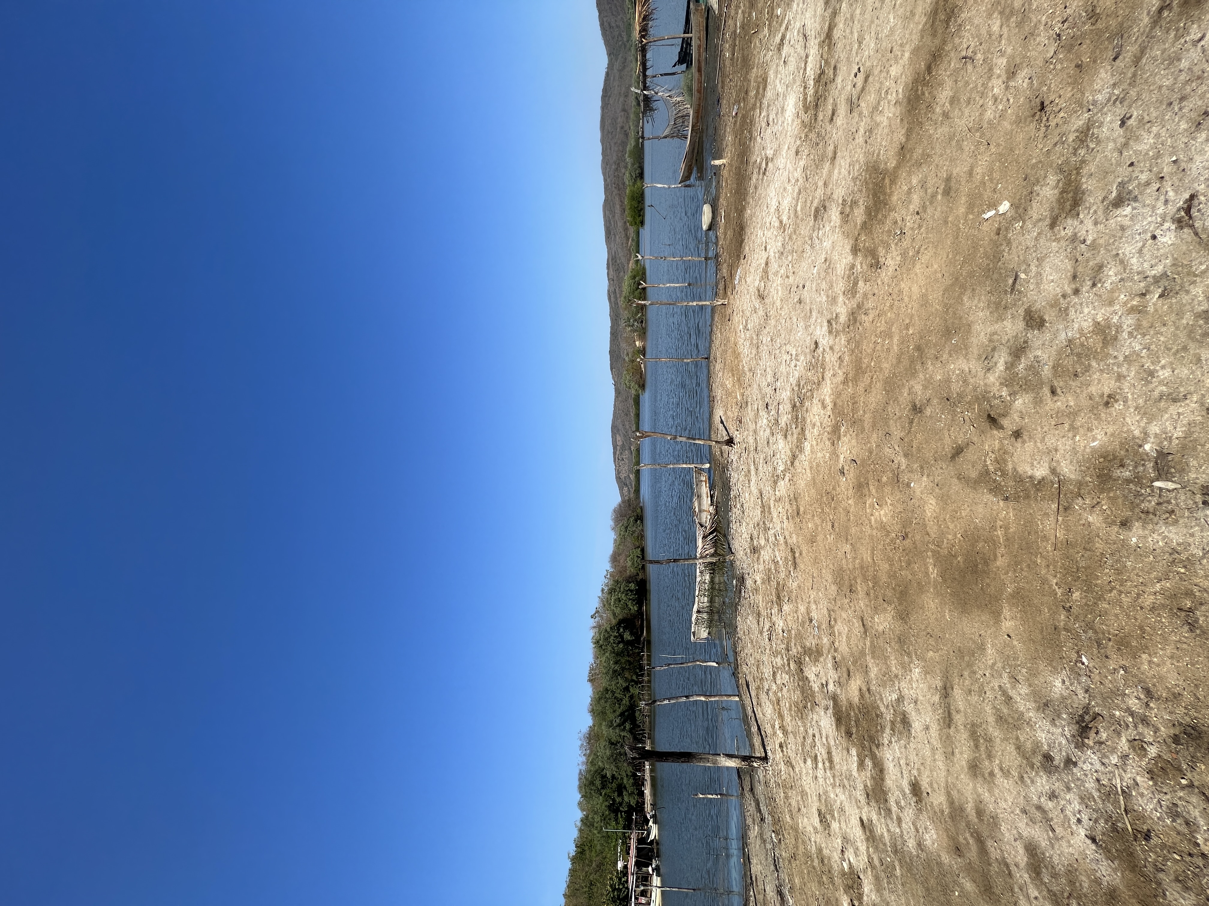
Foto del autor. Minititán, Santiago Pinotepa Nacional, Oaxaca.
Para todxs: datos listos, limpios y públicos.
A pesar de que Google Earth Engine de facilita el acceso a muchos conjuntos de datos, sigue estando la barrera de la accesibilidad, ya que no todo el mundo sabe programar.
Los datos se encuentran en el repositorio de GitHub de N+ Focus, y estan listos para descargar y usar.
Ahí pueden encontrar las anomalías de temperatura, precipitación y la sequía mensual y anual de las entidades y municipios de México. También podrán encontrar el código y la metodología del análisis de los datos.
Anomalía de temperatura máxima de los municipios de México
Visualización hecha directamente con los datos de anomalía de temperatura. No se tuvo que hacer un procesamiento de datos extra para obtener el resultado. La paquetería de Python con la que se hizo fue Altair.
Datos: TerraClimate a través de Google Earth Engine
import altair as alt
import pandas as pd
alt.renderers.set_embed_options(actions=False)

ee_terraclimate_mun_tmmx_url = "https://raw.githubusercontent.com/nmasfocusdatos/desplazamiento-climatico/main/datos/ee_terraclimate_db/ts_mun_year_tmmx_terraclimate.csv"

zero_base_line = alt.Chart(
    pd.DataFrame({'y': [0]})
    ).mark_rule(
        color = "#122451",
        strokeWidth= 1.1,
        strokeDash= [8,8],
        opacity=1
    ).encode(
        y = 'y'
    )

curves = alt.Chart(ee_terraclimate_mun_tmmx_url).encode(
        x = alt.X("year(date_year):T"),
        y = alt.Y("anomaly_tmmx_mean:Q"),
        detail = alt.Detail("cve_geo:N"),
        color = alt.Color("nombre_estado:N").legend(None).scale(scheme="goldorange")
    ).mark_line(
        interpolate = "monotone",
        strokeWidth= 0.5,
        opacity = 0.5
    )

datavis = curves + zero_base_line

datavis_final = datavis.properties(
    width = 980,
    height = 350,
    background = "transparent",
).configure_view(
    stroke = None
).configure_axis(
    title = None,
    labelFont = "Lato, sans-serif",
    tickColor = "#222222",
    tickWidth = 1.3,
    domainColor = "#222222",
    labelColor = "#222222",
    labelFontSize = 15
).configure_axisY(
    ticks = False,
    domain = False,
    labelExpr = "datum.label + ' °C'",
    labelFontWeight = 300,
    gridWidth = 0.1,
    gridColor = "#222222",
    labelPadding = 15,
).configure_axisX(
    grid = False,
    labelFontWeight = 600,
    labelPadding = 7,
    tickCount = {"interval": "year", "step": 5}
)

datavis_final
Eso es todo por ahora
Espero en el futuro se pueda mejorar el análisis con otro tipo de metodología o datos.

Muchas gracias
Escuela de Datos, SocialTIC, Factual y Distintas Latitudes por este espacio.
y también muchas gracias al equipo
Dirección y Subdirección
Omar Sánchez de Tagle e Íñigo Arredondo
Interactivo
Investigación: Saúl Sánchez Lemus y Alberto Pradilla.
Análisis de datos y gráficos interactivos: Isaac Arroyo.
Diseño y desarrollo web: Omar T. Bobadilla.
Video
Realización: Enrique de la Mora, Williams Castañeda y
Rafael López.
Post producción: Jorge Ulloa.
Guión: Cecilia Guadarrama.
Animaciones: Miryam Blancas y Omar T. Bobadilla.
Producción: Aziyadé Sabines.
![]()
… para echar chisme
